
AI for Scaling Microservices: Resource Allocation

If you wait for CPU alerts to fire, you’re already late. I’d treat AI-based scaling as a way to predict demand, set safer limits, and cut waste before cloud spend climbs past $1,000.00 CAD or latency starts missing SLOs.
Here’s the short version:
- I’d use HPA for replica changes, VPA for CPU and memory sizing, and the Cluster Autoscaler for node count.
- For queue-backed jobs, I’d add KEDA so scaling follows backlog, not just CPU.
- I’d feed models with request rate, p95 latency, error rate, queue depth, CPU, memory, and traces.
- I’d start with forecasting for known patterns, test RL only after guardrails are in place, and use service dependency graphs when one bottleneck triggers another.
- I’d keep strict limits on min/max replicas, scale rate, and per-service spend in CAD.
- For teams in Canada, I’d keep metrics, logs, traces, and training data in Canadian regions where policy or law requires it.
A few numbers stand out:
- Dependency-aware scaling cut SLA violations by 41% in one result cited in the article.
- RL-based scaling showed 32% cost reduction or 40% latency reduction, based on target choice.
- One dependency-aware method cut SLO violations by 88% and improved response time by 21%.
What this means for me is simple: AI should sit on top of stable Kubernetes autoscaling, not replace it. I’d begin with clean telemetry, shadow-test forecasts for 2–4 weeks, and roll out to low-risk services first.
| Approach | What I’d use it for | What it needs | Main risk |
|---|---|---|---|
| Native Kubernetes autoscaling | Day-to-day baseline scaling | CPU, memory, custom metrics | Reacts after load shifts |
| KEDA | Queue and event-driven workloads | Queue lag, backlog, trigger data | Poor trigger tuning |
| Forecasting models | Known daily, weekly, or seasonal demand | 30–90 days of time-series data | Bad forecasts from poor data |
| RL | Cost vs latency trade-offs | Guardrails, simulation, audit trail | Unstable scaling if left unchecked |
| Dependency-aware scaling | Multi-service bottlenecks | Traces, service maps, cross-team rules | Harder rollout and ownership |
If I were putting this into production on 2026-08-14, I’d keep the plan plain: fix observability first, set scaling policy from SLOs, test forecasts in read-only mode, then automate bit by bit.
AI Webinar Ep05: Architecting Modern AI Systems: A Microservices Approach
sbb-itb-fd1fcab
The Core Stack for AI-Driven Scaling
AI-driven scaling only works when the base is set up properly. There are five layers in that base: containerised workloads, the Kubernetes control plane, autoscaling controllers, an observability stack, and an AI data pipeline. Each one passes signals to the next, creating a closed loop from raw telemetry to scaling action.
Kubernetes Components That Control Scaling Decisions
Kubernetes has three native autoscaling controllers, and each one works at a different layer of the stack.
HPA (Horizontal Pod Autoscaler) manages replica counts based on CPU, memory, or custom metrics. It fits stateless services like API gateways, frontend services, and idempotent workers, where the simplest way to handle load is to run more instances.
VPA (Vertical Pod Autoscaler) takes a different path. Instead of changing the number of pods, it adjusts pod CPU and memory requests and limits. Use VPA for workloads where CPU and memory needs shift over time, so requests stay right-sized without extra over-provisioning.
Cluster Autoscaler works at the node level. If pending pods can’t be scheduled, it adds nodes. If nodes stay underused, it removes them. That keeps node capacity aligned with demand.
Together, these controllers make up the actuation layer for AI-driven resource allocation.
KEDA extends HPA with scale-to-zero and external event triggers for queue-backed workloads. It connects straight to sources like Kafka topic lag, Azure Queue length, or RabbitMQ depth, and scales pods from queue state instead of CPU. For async workloads like background file processing or overnight batch jobs, that’s often a better match than CPU-only thresholds.
These controllers handle execution. AI sharpens the signals they use.
Observability Data AI Models Need
AI scaling is only as good as the telemetry behind it. For resource allocation, the main signals fall into three groups:
- Infrastructure metrics: CPU millicores, memory RSS, network I/O, and disk throughput
- Application performance metrics: request rate, p50/p90/p99 latency, and HTTP error rate
- Queue and event metrics: queue length, consumer lag, and enqueue/dequeue rate
Business events should also go into the model. That helps it tell the difference between a normal demand pattern and an anomaly.
Prometheus is often used as the Kubernetes metrics collection layer, scraping from kube-state-metrics, node exporters, and application /metrics endpoints. OpenTelemetry gathers distributed traces and spans, time-stamped at nanosecond precision, so models can connect resource pressure to specific service operations. Use ISO 8601 timestamps, such as 2026-08-14T13:45:00-04:00, and keep labels consistent, such as region="ca-central-1".
Data quality matters just as much as data volume. Keep units consistent – CPU in millicores, memory in MiB/GiB, latency in milliseconds. Normalise labels. Filter out deployment-related spikes before training starts. If that prep work is sloppy, the model will learn the wrong patterns. Garbage in, garbage out.
Comparing Scaling Approaches
The table below compares the main scaling options. Pick the mix that suits the workload shape and the level of operating risk.
| Approach | Data Needed | Response Speed | Complexity | Best Fit |
|---|---|---|---|---|
| Native autoscaling (HPA, VPA, Cluster Autoscaler) | CPU, memory, basic custom metrics | Fast | Low | Steady or moderately bursty workloads |
| Event-driven scaling (KEDA) | Queue length, topic lag, external event metrics | Fast | Low–Medium | Asynchronous, queue-backed, or streaming workloads |
| Predictive AI-based scaling | Historical time-series, business events, multi-signal telemetry | Ahead of demand | High | Bursty, seasonal, or dependency-heavy workloads |
In practice, these options don’t cancel each other out. A well-built stack uses HPA for fast replica changes, VPA for gradual right-sizing, Cluster Autoscaler for node capacity, and KEDA for queue-driven services. On top of that, an AI layer can feed custom metrics into HPA or KEDA for proactive scaling.
Use native controllers for baseline scaling, then add AI to forecast demand and tune policy.
The next step is choosing the AI method that turns telemetry into scaling decisions, similar to how AI-powered resource optimization platforms manage complex workforce shifts.
AI Methods Used for Resource Allocation
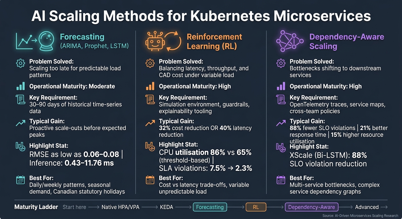
AI Scaling Methods for Kubernetes Microservices: A Side-by-Side Comparison
Once metrics and controllers are in place, the next step is deciding how AI should choose when to scale and what to scale. These methods only make sense when telemetry, scaling controllers, and historical data are already working.
Three AI approaches are practical for microservices scaling today: time-series forecasting, reinforcement learning (RL), and dependency-aware scaling. Each handles a different issue. And each asks for a different level of ops maturity.
Predictive Models for Proactive Scaling
Reactive autoscaling often responds after the damage is done. Forecasting models look a few minutes ahead, which gives the cluster time to scale before users notice slowdowns.
ARIMA fits metrics with steady daily or weekly patterns. Think API request rates that climb between 09:00 and 17:00 local time, or batch ETL jobs that start at 23:00 every night. Prophet is good with seasonality and calendar effects, including Canadian statutory holidays like Canada Day or Thanksgiving. LSTM networks can model non-linear relationships across several signals at once, such as requests, CPU, and queue depth. That helps when load and latency affect each other in ways simpler models miss.
A Prophet + LSTM MAPE loop improved forecasting accuracy over single-model baselines. A predictive ARIMA-based autoscaler for Kubernetes can forecast CPU utilisation about 45 seconds ahead, which gives deployments time to scale before resource exhaustion hits. For teams with moderate ML maturity, lighter models like Holt-Winters or a Kalman filter are a good place to start. One study found they can deliver RMSE as low as 0.06–0.08 with inference times of 0.43–11.76 ms, which is fast enough for real-time scaling decisions.
The minimum setup here is plain but strict: reliable observability, a stable Kubernetes autoscaling setup, and basic MLOps for retraining and deployment. In practice, that usually means 30–90 days of steady Prometheus metrics so the model can learn weekday versus weekend patterns and monthly cycles. Store time-series data in Canadian cloud regions such as AWS ca-central-1 or GCP northamerica-northeast1 to support data residency requirements.
Forecasts should feed Kubernetes scaling actions, not replace them.
Reinforcement Learning for Policy Optimisation
Rule-based autoscaling can make it tough to tune performance and cost at the same time. RL helps with that trade-off by learning a policy that balances both over time. The agent watches system state – current replicas, CPU utilisation, p95 latency, estimated cost in CAD – and then picks an action such as scale up, scale down, or hold to maximise a long-term reward.
Use a reward function that penalises p95 latency, error rate, and CAD cost.
Guardrails are not optional in production. Set hard replica minimums and maximums, limit how fast replica counts can change, and enforce daily CAD spend caps per service. For example, no more than ±5 pods per 5 minutes is a sensible rate limit.
RL sits on top of existing autoscaling controllers. It sharpens the signals they use instead of replacing them. When it works, the gains are hard to ignore. One RL-based autoscaler achieved either 40% latency reduction or 32% cost reduction, depending on the optimisation target. Another reached 86% CPU utilisation versus 65% for threshold-based policies, while SLA violations fell from 7.5% to 2.3%.
That said, RL asks for a lot more from the platform team: mature observability, simulation, guardrails, and explainability tooling so SRE teams can audit why the agent made a given decision. Start pilots on non-critical workloads first, like background processing or internal tools, before moving to customer-facing services.
RL becomes useful only after the baseline autoscaling loop is stable.
Multi-Service Scaling Based on Dependencies
Scaling one service on its own often just shifts the bottleneck somewhere else. Dependency-aware scaling deals with that by treating connected services as a group instead of separate targets.
Use traces to build a service graph that shows how load moves across APIs, queues, databases, and workers. That graph ties straight into the observability stack described earlier – OpenTelemetry traces and service maps feed the dependency model. Scaling policies can then coordinate actions across services. If incoming queue depth rises, scale both the API and its downstream worker services together. If traces show database latency climbing under peak API load, scale the cache layer ahead of time.
Spatio-temporal graph neural networks (GNNs) push this further by modelling how workload patterns move across the service graph over time. The XScale algorithm, which uses Bi-LSTM forecasting with dependency awareness, reduced SLO violations by 88%, increased resource utilisation by 15%, and cut average response time by 21% compared to advanced reactive methods. To do this in practice, teams need mature observability: OpenTelemetry traces, service maps, and agreed cross-service scaling policies with clear ownership boundaries.
| Method | Problem It Solves | Operational Maturity Needed | Typical Gain |
|---|---|---|---|
| Forecasting (ARIMA, Prophet, LSTM) | Scaling too late for predictable load patterns | Moderate: stable history and basic retraining. | Proactive scale-outs before expected peaks |
| Reinforcement learning | Balancing latency, throughput, and CAD cost under variable load | High – simulation, guardrails, explainability tooling | 32–40% cost or latency improvement |
| Dependency-aware scaling | Bottlenecks shifting to downstream services | High – distributed tracing, service graphs, cross-team policies | 88% fewer SLO violations |
Next, convert the chosen method into Kubernetes metrics, guardrails, and rollout controls.
Implementation Plan for Kubernetes and Cloud Environments
Production success has less to do with picking the "best" model and more to do with getting the basics right: low-cardinality metrics, consistent units, and stable baselines. AI-assisted scaling only starts to work once that base is steady. If your metrics are messy, your requests are off, or HPA behaves unpredictably, every layer you add after that gets shakier.
That’s why instrumentation comes first. Every control that follows depends on it.
Instrument Services and Define the Right Metrics
Give each microservice a Prometheus-compatible /metrics endpoint. Then expose metrics that show actual demand, not just system strain. http_requests_total, request duration histograms, queue depth, and job throughput tell you much more than raw CPU alone.
These metrics help drive:
- Replica counts
- Request sizing
- Node capacity
Keep labels low-cardinality. Use tags like namespace, service, version, and region such as ca-central-1. Skip per-user or per-request labels. They blow up metric storage and slow query performance.
Size requests from P90 usage. A good pattern is to run VPA in recommendation mode for two to four weeks, check the output in staging, and only then apply it in production. Set each scaling target from an SLO, like P95 latency under 250 ms or queue drain time under five minutes.
Once your metrics are dependable, use them to put guardrails around scaling behaviour instead of trying to brute-force overrides.
Add Event-Driven and Predictive Scaling Safely
After metrics and requests are stable, bring in event-driven and forecast-based controls.
If HPA is already stable on custom metrics, add KEDA to read queue signals and adjust replica counts from discrete triggers. Set cautious minReplicas and maxReplicas limits for each service. Add cooldown periods too: no scale-down within five to ten minutes of a scale-up. Pair that with step-wise changes so you don’t get thrashing.
For predictive scaling, start in forecast-only mode. Shadow-test it for two to four weeks against live traffic patterns. Put hard limits on replica counts and error rates, then allow live changes on one non-critical service first. After that, expand service by service.
This is one of those cases where slow is smart. A quiet rollout beats a noisy incident.
Cost Reporting and Operating Standards for Canada
Scaling should show up in CAD spend, not just cluster telemetry.
Pull cloud billing data into internal dashboards, convert it to CAD, and group it by Kubernetes namespace and service. That breakdown makes it much easier to spot whether scaling choices are over-allocating or under-allocating resources. Use 1,234.56 CAD formatting, and annotate dashboards with scaling events so teams can tie each change to what it cost or saved.
Use ISO 8601 timestamps with 24-hour time across logs and runbooks, such as 2026-08-14T09:00:00-04:00. That avoids confusion across provinces and makes cross-region troubleshooting much easier. Stick to metric units throughout: CPU in millicores, memory in MiB/GiB, and network in Mbit/s. For federal regulated workloads, keep logs, metrics, and replicas within Canada to meet residency rules.
Baseline with HPA first. Then add custom metrics. After that, layer in KEDA or predictive scaling only where the workload shape makes it worth the extra control.
Governance, Risks, and Conclusion
Once AI starts making scaling decisions, governance is what keeps those decisions safe, auditable, and compliant.
Common Failure Points and Control Measures
Even well-built AI scaling systems tend to fail in a few familiar ways. One of the biggest is delayed telemetry. When metrics show up late, the autoscaler reacts to old demand instead of current demand. The result? Users hit latency spikes even though the system did, on paper, respond. A better approach is to scale from work-intake signals like request rate, queue depth, and concurrency instead of leaning on CPU alone, since CPU is a trailing signal.
Another common problem is thrashing. Reinforcement learning can cut latency and reduce pod count, but if you don’t set firm minReplicas and maxReplicas limits, it can still send the system bouncing up and down. Rate-limiting scaling actions helps calm that pattern down.
Then there’s the quieter risk: poor training data. It’s easy to miss, and it can do just as much damage. If a model is trained on off-peak traffic or a narrow time window, it may misread demand surges during events like Black Friday or tax season filing periods. Keep production and test telemetry separate. Test against traffic patterns that reflect Canadian usage. Add confidence scoring, and trigger automatic rollback when health metrics start to slip.
These controls lower technical risk. After that, the next issue is simpler: where the data lives, and where the decisions are allowed to happen.
Canadian Compliance and Data Residency Considerations
For regulated workloads, the observability pipeline itself can hold regulated data. Metrics, logs, traces, and training datasets may include IP addresses, session IDs, or system details. In those cases, the data may need to remain in Canadian regions under PIPEDA or provincial privacy law.
Government of Canada sovereignty guidance treats foreign access as a risk for Canadian AI workloads. That means region rules shouldn’t be left to chance. Set those constraints by default in Terraform and Helm. It also helps to log the model version, training data, and approver tied to each scaling decision. Those records make internal reviews easier and support external regulatory reporting when needed.
With those controls and residency rules in place, the main adoption question shifts from can this work? to how far should rollout go right now?
Key Takeaways for Adoption
AI-driven resource allocation tends to pay off most when demand changes a lot, services have many dependencies, or over-provisioning gets expensive in CAD. But it does add complexity. So it should sit on top of strong observability and stable baseline autoscaling, not try to replace them.
A smart starting point is decision support. Let the model suggest scaling actions, but keep human approval in the loop. From there, move into automation step by step, starting with non-critical services. For organisations in regulated sectors, critical government, healthcare, or financial workloads should be the last place you hand over full control, not the first.
Digital Fractal Technologies Inc helps Canadian teams design compliance-aware microservices, telemetry pipelines, and AI-driven scaling controls.
FAQs
When should AI scaling be added to Kubernetes?
Add AI-driven scaling to Kubernetes when traffic is bursty, uneven, or hard to predict. It works well for e-commerce sites during seasonal rushes, government portals that spike around deadlines, and apps that get hit during live events or campaign launches.
Instead of relying on static deployments, this approach uses predictive signals or live metrics to scale workloads up or down as demand changes. That means better use of compute resources and tighter control over cloud spend, especially when over-provisioning can push costs up by as much as 30%.
What data is needed for predictive microservice scaling?
Predictive microservice scaling uses past trends and live usage data to estimate resource needs before demand spikes hit.
The main inputs include historical usage patterns, seasonal trends, CPU usage, memory consumption, request rates, latency, queue depths, and event throughput. When you line up that telemetry with application performance data, you get a clearer picture of what’s coming next.
That makes resource allocation more proactive and efficient – instead of reacting after performance starts to slip.
How can AI scaling be rolled out safely?
Use a phased, incremental approach. Start with the busiest bottlenecks first, but try scaling patterns on lower-risk services before rolling them out more broadly.
Set clear SLIs and SLOs, and watch them on an ongoing basis. Use anomaly detection to catch deviations early and trigger rollbacks or circuit breakers when needed. As the architecture changes over time, keep human oversight, documentation, and runbooks in place.