
Case Study: Observability in ML Pipelines
If your ML dashboard looks fine but users still get bad predictions, you do not have enough visibility.
I see one clear lesson in this case: teams need comprehensive development solutions to track data, model behaviour, infrastructure, and cost at the same time. In this example, better tracing and alerting helped cut detection time from 4.2 hours to 11 minutes, cut resolution time from 3–5 days to 12 minutes, and spot drift 2 weeks early. It also helped reduce failed deployments, lower false alarms, and avoid wasted GPU spend of about C$3,000 per month.
Here’s the short version:
- The main problem: standard dashboards showed CPU and GPU health, but missed bad data, drift, training-serving skew, and request-level delays.
- What changed: the team linked OpenTelemetry trace IDs with MLflow run IDs so each production issue could be tied back to the exact training run.
- What they watched: schema drift, null rates, row drops, confidence scores, latency split by
queue_wait_msandforward_pass_ms, GPU usage, and cost per inference in C$. - What improved: MTTD, MTTR, deployment speed, trust scores, and alert quality.
- What I’d take from it: set baselines in the first 30 days, add alerts for failure paths, and make audit trails part of the pipeline from day one.
This case shows a simple point: ML systems fail in places that infra metrics alone cannot show, and that is where observability starts to matter.
The Baseline Pipeline and the Gaps That Caused Incidents
Pre-Observability Pipeline Architecture
Before observability was in place, the pipeline was mostly manual. Training data lived in local or shared folders, features were built in notebooks, and models were copied into a shared directory so someone could restart things by hand. Online inference ran through a basic FastAPI service.
The path from ingestion to feature prep, training, validation, and serving wasn’t documented. There was no link between a training run and the exact data snapshot used to produce it. So when something went wrong, engineers couldn’t trace a bad prediction back to its source with any confidence.
Put simply, the setup had no dependable trail from raw data to the model running in production.
Missing Visibility Across Data, Model, and Infrastructure
The blind spots showed up across data, model behaviour, and infrastructure.
On the data side, there were no schema checks, no null-value gates, and no monitoring for feature distributions. The feature store also wasn’t returning values matched to inference time, which meant training-serving skew slipped by without any warning. If an input was corrupted or had shifted, it could move through the pipeline without a single automated alert.
On the model side, there was no drift detection and no record of experiment lineage. Hyperparameters and metrics were tracked in spreadsheets. If model quality got worse little by little, there was no signal to catch it. The system would keep serving predictions that looked fine at a glance but were wrong in behaviour. That kind of failure is easy to miss. Narrow accuracy metrics were not enough to catch drift or data-quality failures.
On the infrastructure side, the team did have CPU and GPU utilisation dashboards. The problem was that those numbers told only part of the story. A GPU can show 75% utilisation and still hold everything up if requests spend 60% of their time waiting for GPU memory to free up, which standard metrics don’t show. Logs were also split across the API layer, the feature store, and the model server, with no trace IDs to tie them together.
Incidents That Exposed the Problem
These gaps didn’t stay hidden for long. They showed up in two production incidents.
The first came from an incorrect data snapshot. Users noticed weaker predictions before the versioning error was found, and by then the model had already been serving bad outputs for nearly three weeks. The incident was tied to about C$150,000 in revenue impact.
There was also no drift-triggered retraining, so the model stayed exposed to seasonal demand shifts.
Here’s the short version of what was missing and what each gap hid:
| Missing Signal | What It Hid | Consequence |
|---|---|---|
| Schema validation | Corrupted inputs reaching the model | Silent bad predictions |
| Data versioning | Which snapshot trained which model | ~200 engineer-hours spent debugging version errors |
| Drift detection | Seasonal distribution shifts | Stale model serving through changing demand |
| Distributed tracing | End-to-end request trace across API, feature store, and model server | Hours of manual root-cause analysis |
| GPU queue time | Requests stalled waiting for GPU memory | High latency despite "healthy" utilisation metrics |
sbb-itb-fd1fcab
Observability Architecture and Implementation
Target Design for End-to-End ML Observability
After the incidents, the team made a practical call: instrument the stack they already had instead of rebuilding everything.
They used OpenTelemetry (OTel) for traces and metrics, and MLflow for experiment tracking. That gave them observability across the ML stack without swapping out core parts.
The key move was simple but powerful: link the OTel Trace ID to the MLflow Run ID. So every production trace points back to the exact experiment run behind that model.
That means if something goes wrong in production, the team doesn’t have to guess which training run caused it. They can go straight from live telemetry to the run, data, and settings tied to that model.
They rolled this out in layers. First came the two steps most likely to fail: data loading and model training. After that, they extended instrumentation to preprocessing and evaluation.
Signals, Alerts, and Automated Response
Once the trace-to-run link was in place, alerts could point to the exact data, model, and infrastructure conditions behind each issue.
| Layer | Key Signals | Alert Type |
|---|---|---|
| Data | Freshness, null rates, schema drift, row drop rate | Threshold-based |
| Model | Confidence scores, prediction distribution, p95 latency, throughput | Anomaly/Drift-based |
| Infrastructure | GPU compute utilisation, VRAM usage, CPU, thermal status | Threshold-based |
| Business | Cost per inference (C$), token/cost ratio, ROI | Trend-based |
On the data side, the rules were clear. A drift score above 0.3 on key features triggers an alert, and null rates above 5% are flagged right away.
On the infrastructure side, GPU utilisation above 95% for 10 minutes sends a page.
The team also split inference latency into queue_wait_ms and forward_pass_ms. That sounds minor, but it matters. It separates waiting in line from actual model compute time, which makes triage much less messy.
Automated response was tied to quality gates too. Responses with a groundedness score below 0.90 go to human review. Slack alerts include a direct link to the trace, so the engineer on call can jump straight into triage instead of digging through tools first. And when drift thresholds are crossed, retraining starts automatically rather than sitting around until the next scheduled review.
"To be honest, I’ll put monitoring before latency. I don’t mind waiting for a response for more than five seconds. But if you have a really bad model that gives terrible predictions, you will lose far more money." – Dayle Fernandes, MLOps Engineer, DeepL
For baselines, the team used the first 30 production days to learn normal behaviour, then alerted on drift from those baselines.
Before-and-After Observability Comparison
This wasn’t just about seeing more. It changed how fast the team could act.
| Dimension | Before | After |
|---|---|---|
| Data visibility | Silent failures; no null-rate or schema monitoring | Real-time tracking of null rates, row counts, and schema drift |
| Incident detection | User-reported or manual audits | Automated threshold and anomaly alerts |
| Root-cause analysis | Manual correlation across fragmented logs | Trace-level analysis |
| Model performance transparency | Black-box execution; no drift signal | Confidence score distributions and drift scores in live dashboards |
| Business impact measurement | Hidden costs discovered after the fact | Cost-per-inference tracking and quality gating before delivery |
Towards Observability for Machine Learning Pipelines
Incidents After Implementation and Measurable Results
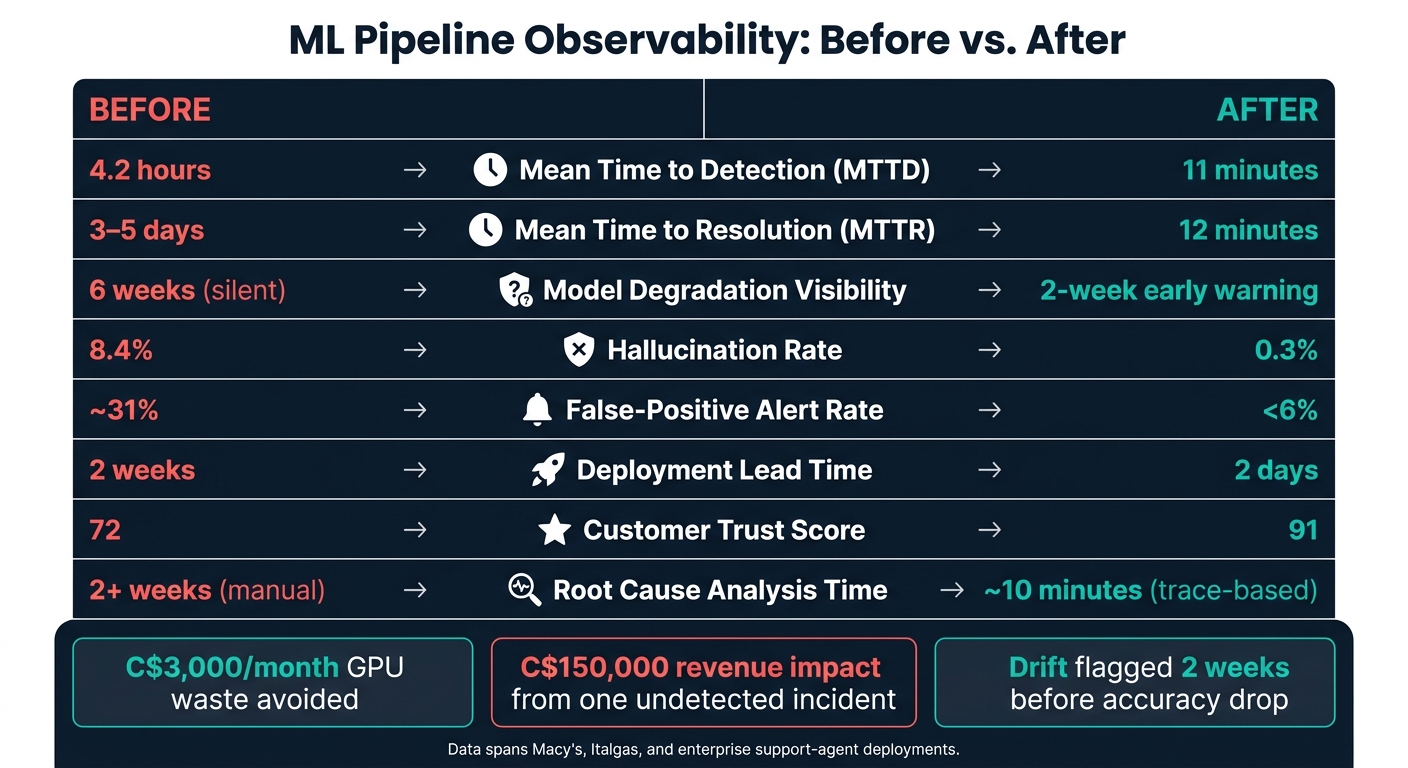
ML Pipeline Observability: Before vs. After Key Metrics
How Observability Changed Detection and Diagnosis
Across three deployments, observability turned silent pipeline failures into incidents teams could trace and fix.
In one production data pipeline at Macy’s Systems & Technology, the CDC feed went silent from a regional distribution centre. Before observability, that kind of failure would have stayed hidden for an average of 4.2 hours. This time, the system caught a 62% drop in orders_daily_fact volume within 11 minutes and suggested replaying the last known good state. The team fixed the issue before the 6:00 AM business reporting deadline.
At Italgas, a fraud detection model showed a PSI of 0.31 in merchant_category. The observability system flagged the feature drift two weeks before accuracy would have fallen. It traced the root cause to a new payment provider that had not been mapped correctly in the pipeline.
The pattern is hard to miss: faster signal, faster diagnosis, and far fewer silent failures.
Operational and Business Outcomes
Across deployments, observability cut detection time, resolution time, and alert noise in a big way.
MTTD dropped from 4.2 hours to 11 minutes. In the enterprise support-agent case, MTTR for quality issues fell from 3–5 days to 12 minutes. Automated quality scoring cut hallucinations from 8.4% to 0.3%, while customer trust scores climbed from 72 to 91.
Adding business context to the observability layer also reduced false-positive alert rates from about 31% to under 6%.
Results Comparison Table
The biggest gains showed up in three places: faster detection, faster recovery, and less alert noise.
| Metric | Pre-Observability | Post-Observability |
|---|---|---|
| Mean Time to Detection (MTTD) | 4.2 hours | 11 minutes |
| Mean Time to Resolution (MTTR) | 3–5 days | 12 minutes |
| Model Degradation Visibility | 6 weeks (silent) | 2-week early warning |
| Hallucination Rate | 8.4% | 0.3% |
| False-Positive Alert Rate | ~31% | < 6% |
| Deployment Lead Time | 2 weeks | 2 days |
| Customer Trust Score | 72 | 91 |
| Root Cause Analysis Time | 2+ weeks (manual) | ~10 minutes (trace-based) |
Figures span Macy’s, Italgas, and the support-agent case study.
These results point straight to the implementation choices that mattered most when building a digital transformation roadmap.
Lessons Learned and Conclusion
What the Team Would Do Earlier Next Time
These results point to three clear lessons for teams building ML pipelines. The big one is simple: build observability in from the start. Don’t bolt it on after the first outage.
Link OpenTelemetry trace IDs to MLflow run IDs on day one. That makes root-cause analysis much shorter after bad predictions or failed deployments, because teams can connect live telemetry straight to the training run behind the model.
Set production baselines within the first 30 days. And don’t stop at the happy path. Traceability only helps if the failure path is instrumented too, so teams should track fallbacks, timeouts, and exceptions on purpose.
Practical Recommendations for Canadian Organizations
For Canadian teams, these same ideas need to fit local budget and governance needs. Cost dashboards should report spend in C$, with cost-per-inference and projected month-end spend tied to departmental budgets. A good rule is to keep the observability stack’s total cost under 5–10% of the infrastructure it monitors.
Logs and traces also work as audit trails, which matters for Canadian data governance requirements. Using vendor-neutral standards like OpenTelemetry gives teams portability, so they can change backends without re-instrumenting the entire codebase.
Key Takeaways from the Case
One pattern shows up again and again: silent failures are the main risk. The gains came from watching infrastructure, data, model behaviour, and cost together. Miss one layer, and you leave a blind spot.
FAQs
What is ML observability?
ML observability gives teams end-to-end visibility across the machine learning lifecycle. It goes past basic monitoring by tracking data quality, feature health, model behaviour, and resource performance so teams can keep systems reliable.
With tools like OpenTelemetry and MLflow, teams can catch problems such as data drift, schema changes, and latency bottlenecks before they hit production.
Why are infra metrics alone not enough?
Infrastructure metrics tell you if a machine is up and running. They do not tell you if your ML output is correct.
That gap matters more than many teams expect. CPU, RAM, and disk can all look healthy while data drift, schema changes, or logic errors quietly push out bad results with no alert at all.
There’s another issue: these metrics are usually aggregated. So you lose the story behind individual requests. And that missing context can hide problems until they start affecting users.
That’s why infrastructure monitoring works best when it’s paired with data and model-level observability.
How do we start adding observability?
Start small instead of rebuilding the whole system at once.
A good first move is experiment tracking with tools like MLflow or W&B. That gives you fast visibility into training runs and models without forcing major infrastructure changes. You can see what was tested, what changed, and what worked – without turning the setup upside down.
For pipeline and infrastructure monitoring, standardize instrumentation with OpenTelemetry. Begin with auto-instrumentation for system and process metrics. After that, add custom spans for ML-specific context like data quality, feature health, and inference latency.
This approach keeps the work practical. You get useful signals early, then layer in deeper ML context as the setup matures.