
Edge Anomaly Detection Flags Locally Before Cloud Review

The pattern that holds up in production is edge triage paired with cloud confirmation: lightweight on-device models like VARADE or quantized autoencoders flag candidates using TensorFlow Lite, ONNX Runtime, or OpenVINO, then forward only the suspicious cases to the cloud for heavier scoring. The edge model is tuned for recall so it rarely misses a real event, and the cloud model is tuned for precision so it filters the false alarms that recall-first thresholds inevitably produce.
TL;DR:
- On ESP32 devices, isolation forest ensembles can train in 1.2 to 6.4 seconds, infer in under 16 milliseconds, and use about 80 KB of RAM.
- Eight bit quantization can shrink models roughly fourfold, but test converted artifacts on target devices because calibration and decision boundaries can shift.
- Log raw scores for a week before setting thresholds; tune edge detection for recall, and delay low confidence alerts until a second window confirms them.
- Run new models in shadow mode for at least one full operational cycle, then canary them while monitoring latency, memory, detection metrics, and rollback readiness.
Table of Contents
- The Real-Time Edge Anomaly Detection Pipeline: Stages and Responsibilities
- Edge-Friendly Model Families and Architectures
- Model Optimization and the Edge Runtime Toolchain
- Training and Update Strategies for Distributed Edge Fleets
- Edge-to-Cloud Architecture Patterns and Trade-offs
- Evaluation, Benchmarks, and Metrics to Report
- Security, Platform Trust, and Operational Controls
- Representative TinyML and Industrial Deployment Examples
- Practitioner Checklist for Prototyping and Deploying Edge Anomaly Detection
- How We Think About Edge Anomaly Detection Projects
- AI Readiness Audit and Edge Integration With Digital Fractal
- FAQ
- Sources
The Real-Time Edge Anomaly Detection Pipeline: Stages and Responsibilities
A working edge anomaly pipeline splits cleanly into stages, and deciding which stage runs on the device versus the gateway or cloud is the first architectural choice that determines everything downstream. Get this split wrong and you either starve the device of compute or flood the network with raw telemetry it was never designed to carry.
- Ingestion: sensors or cameras stream raw signal at a fixed sampling rate; buffering must respect the device’s RAM budget, often under 256 KB on microcontroller-class hardware.
- Preprocessing: filtering, normalization, and windowing turn raw samples into fixed-size slices the model can consume, typically sliding windows of a few hundred milliseconds to a few seconds depending on the signal.
- Feature extraction: either handcrafted statistics (mean, variance, spectral features) for classical models, or a learned embedding layer for autoencoders and transformers.
- Inference: the on-device model scores the window and produces an anomaly score or probability, ideally in under 20 milliseconds to keep pace with streaming data.
- Decision: a threshold or ensemble rule decides whether the score warrants local action, silent logging, or escalation.
- Escalation: flagged windows, along with compact metadata, travel to the gateway or cloud for a second opinion.
- Model update: periodic retraining or federated aggregation refreshes the on-device model without requiring a full redeployment cycle.
Each stage carries its own constraint. Ingestion and preprocessing are CPU-bound and must fit inside whatever duty cycle the device’s power budget allows; a battery-powered sensor can’t afford continuous full-rate sampling if its anomaly rate is naturally low. Feature extraction and inference are memory-bound, which is why model families are chosen by hardware class rather than accuracy alone. Decision logic is the cheapest stage computationally but the one most often under-engineered: a naive fixed threshold generates alert fatigue, while a poorly tuned ensemble buries real events in noise.
When a window escalates, the payload should carry more than the raw score. Useful metadata includes a timestamp, the feature embedding (not just the raw window, which saves bandwidth), a device health snapshot (battery, temperature, clock drift), and a model version identifier so the cloud side knows which detector produced the flag. That last detail matters more than it sounds: fleets running mixed model versions during a staged rollout need traceable provenance for every escalation.
Tiny-MLOps extends standard MLOps practice to this constrained environment: automated conversion pipelines, on-device sanity checks before a model ships, and staged rollout with rollback paths are what separate a research prototype from something you can run across thousands of devices without someone driving out to recover a bricked unit, a pattern documented in recent TinyML anomaly detection work. The same operational discipline shows up in broader real-time IoT analytics pipelines, where telemetry handling and update cadence follow similar constraints even outside anomaly detection specifically.
Edge-Friendly Model Families and Architectures
Model choice at the edge is a hardware conversation first and an accuracy conversation second. The same model that produces state-of-the-art results on a GPU cluster is frequently unusable on a microcontroller, so practitioners map families to hardware classes rather than picking one architecture and hoping it compresses.
- MCU-class devices (ESP32, Cortex-M series): isolation forest ensembles and tiny autoencoders dominate here. A published prototype trained an unsupervised isolation forest directly on an ESP32 microcontroller, with training times of a few seconds and inference under 16 milliseconds using a small memory footprint.
- SBC and SoC-class devices (Raspberry Pi, embedded SoCs): this is where variational autoregressive models and lightweight transformer variants fit. VARADE targets this exact tier, balancing probabilistic scoring against the tighter compute budget of single-board hardware.
- Jetson-class devices (embedded GPUs): optimized deep learning models, including quantized transformers, become viable. VARADE++ reports a favorable accuracy versus inference-frequency trade-off specifically on Jetson-class hardware, achieving competitive AUC-ROC while sustaining inference rates suited to real-time streams.
Forecasting and autoregressive approaches suit streaming multivariate time series anomaly detection (MTSAD) because they predict the next value and flag deviation from that prediction, which naturally adapts to slowly drifting baselines. Their limit is sensitivity to sudden regime changes: a legitimate operational shift, like a machine starting a new production run, can look identical to an anomaly until the model has a few windows to adjust. Variational variants address this by outputting predictive variance alongside the point estimate, and that variance can serve directly as the anomaly score, which tends to be more robust than raw forecasting error on constrained models.
For video and other high-dimensional streams, embedding plus local kNN triage is the practical pattern. Instead of running a full detection model per frame, the device computes a compact embedding and compares it against a small local index of known-normal embeddings using k-nearest-neighbor distance. This avoids running a heavy model per frame while still catching novel patterns, and it is the basis for edge shard designs used in production video pipelines.
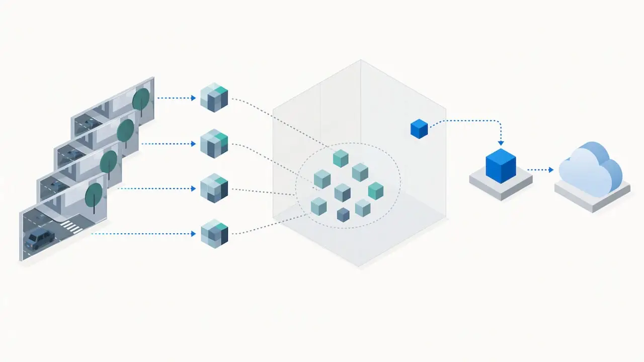
Setting the operating threshold is where most deployments actually fail, not model selection. A threshold tuned on a clean validation set rarely survives contact with real sensor drift, seasonal patterns, or hardware aging. The practical fix is to tune the edge threshold for recall, accept a higher false-positive rate locally, and let the cloud-side ensemble apply the precision filter. Variance or uncertainty outputs from variational models help here directly: a high-confidence anomaly score can escalate immediately, while a low-confidence one can wait for a second window before triggering an alert.
Pro Tip: Log raw anomaly scores for a week before setting any production threshold. Drift in the score distribution during that window often reveals more about sensor behavior than any model metric will.
Teams building vision-based detectors on constrained hardware face similar trade-offs to the ones covered in our guide to lightweight edge object detection models, where model compression and embedding-based matching follow the same hardware-first logic.
Model Optimization and the Edge Runtime Toolchain
Getting a model small enough to run on constrained hardware is a separate engineering problem from training it, and it has its own workflow: export, quantize, validate, measure, then ship.
- Post-training quantization converts 32-bit floating point weights to 8-bit integers (or mixed precision) after training, typically cutting model size by roughly 4x with a small, measurable accuracy cost that varies by architecture.
- Mixed-precision strategies keep sensitive layers at higher precision while quantizing the rest, useful when full int8 quantization degrades a model’s anomaly score calibration.
- Format conversion flow: export the trained model to a standard format, quantize it, run on-device validation against a held-out test set, then gate the release through a Tiny-MLOps pipeline that checks latency and memory before allowing a fleet-wide push.
- On-device validation should test the actual converted artifact, not the pre-conversion model; quantization occasionally shifts decision boundaries in ways that only show up after conversion.
Runtime choice depends on target hardware more than personal preference. TensorFlow Lite has the broadest support across microcontrollers and single-board computers and is usually the first conversion target for a new project. ONNX Runtime trades some of that MCU-level reach for hardware portability: a model exported once can run across CPUs, GPUs, and several accelerator types without separate conversion paths. OpenVINO is the choice when the deployment target is Intel hardware specifically, since it exploits Intel’s instruction sets and integrated accelerators more directly than the general-purpose runtimes do. Together these three form the practical toolchain for nearly every edge anomaly project, a pairing reflected across current edge runtime documentation and deployment case studies.
TinyML prototypes have reported inference under 16 milliseconds and roughly 80 KB RAM using an isolation forest ensemble on an ESP32 microcontroller, which gives a concrete baseline for what “lightweight” means in practice on MCU-class hardware.
After conversion, measure three things on the actual target device, not a development machine: inference latency under realistic load, peak memory during inference (not just model size), and power draw per inference cycle if the device runs on battery. Report all three together, since optimizing one in isolation often regresses another, a quantized model that shrinks memory but increases latency on certain accelerators is a common surprise worth catching before fleet rollout.
Training and Update Strategies for Distributed Edge Fleets
Keeping a fleet of edge models current without shipping full retrains to every device is one of the harder operational problems in this space, and the answer usually combines federated learning with lightweight on-device adaptation.
- Federated learning lets each device train locally on its own data and share only model updates, not raw data, with a central aggregator, which helps with privacy and bandwidth but introduces a convergence problem.
- Non-IID data handling: devices in different locations or operating conditions see different data distributions, and a 2025 systematic review of federated learning in edge environments found that this heterogeneity remains a major bottleneck for convergence; the review recommends asynchronous updates and selective update mechanisms as practical mitigations.
- Asynchronous and selective updates: rather than waiting for every device to submit an update on a fixed schedule, aggregating updates as they arrive and selectively weighting contributions from devices with more representative data improves stability in heterogeneous fleets.
- Cluster-level training: grouping devices by operating profile before aggregation, rather than treating the whole fleet as one population, reduces the damage non-IID data does to the shared model.
- On-device rapid retraining: for TinyML-scale models, full retraining can complete in single-digit seconds, isolation forest ensembles in the ESP32 prototype retrained in roughly 1.2 to 6.4 seconds, which makes local adaptation to drifting baselines practical without a round trip to the cloud.
- Shadow mode and canary rollout: a new or retrained model runs alongside the production model, scoring the same data without acting on it, before a small percentage of the fleet receives the update live.
- Rollback: every update ships with a path back to the previous known-good model, triggered automatically if canary metrics degrade beyond a defined tolerance.
Concept drift, the slow shift in what “normal” looks like over time, is the practical reason update strategies matter at all. A model trained once and frozen will drift out of calibration within weeks on most industrial signals, whereas a fleet that supports rapid local retraining or federated refresh can track that drift without constant manual intervention. The combination of fast on-device retraining for immediate local correction and periodic federated aggregation for fleet-wide consistency covers both time scales.
Edge-to-Cloud Architecture Patterns and Trade-offs
The two-tier triage pattern, recall-oriented edge plus precision-oriented cloud, is the dominant architecture for a reason: it matches each tier’s strength to what it’s good at and avoids forcing either side to do a job it’s not suited for.
- Two-tier triage: the edge model runs continuously and escalates anything above a deliberately loose threshold, while the cloud model rescores escalations with heavier compute and tighter precision requirements; pick this pattern whenever bandwidth or edge compute makes full-fidelity scoring on-device impractical.
- Immutable versus mutable shards: a documented pattern from a video anomaly edge-to-cloud pipeline splits the local index into an immutable baseline shard, representing established normal behavior, and a mutable live-context shard that absorbs recent data; this keeps the baseline stable while still adapting to short-term context.
- Snapshot sync: periodically syncing the mutable shard back to a central store, rather than streaming every update, keeps bandwidth predictable and gives the fleet a consistent recovery point if a device needs to rebuild its local index.
- Bandwidth and cost trade-offs: the same pipeline reported roughly a 6x reduction in cloud bandwidth by escalating only triaged candidates instead of streaming raw data, while maintaining around 95% recall at the edge, with the cloud ensemble handling the resulting false positives.
- Offline resilience: pinned anomalies (flagged events held locally until confirmed), upload queues that buffer escalations during connectivity loss, and defined retention windows that drop the oldest unconfirmed events first keep the system functional when the link to the cloud drops.
- Escalation logic design: combining a simple threshold with ensemble scoring and temporal boosting, where repeated flags on the same window within a short period raise confidence faster than an isolated flag, reduces both missed events and false escalations.
The underlying trade-off is intentional, not a compromise: edge triage accepts more false positives in exchange for near-complete recall, because missing a real anomaly is usually far costlier than a wasted cloud rescoring cycle. This is the same framing covered in our broader comparison of edge versus cloud AI workload placement, where the decision of what runs where follows cost and latency constraints rather than a fixed rule.
Evaluation, Benchmarks, and Metrics to Report
Reporting the right metrics, measured the right way, is what separates a detector that looks good in a notebook from one that survives a stakeholder review after a missed incident.
- Detection metrics: AUC-ROC and F1-score remain the standard pair, AUC-ROC for threshold-independent discrimination and F1 for a specific operating point; report both, since a model can have strong AUC-ROC and still perform poorly at the threshold you actually deploy.
- Runtime metrics: inference frequency in Hz, end-to-end latency in milliseconds, and peak memory footprint all need to be measured on the target device, not a development workstation.
- Benchmark datasets: SWaT and WADI test industrial control system scenarios with physical process dynamics, SMD covers multivariate server machine telemetry, and HDFS tests log-based anomaly detection; together they cover the main data modalities edge detectors encounter.
- Experiment structure: fix the latency budget first (what your use case actually tolerates), then test windowing and throughput against that budget rather than optimizing accuracy in isolation and hoping it fits afterward.
Lightweight transformer variants have reported high F-scores across typical industrial benchmarks while remaining compatible with mixed-precision quantization for edge deployment, according to recent work on transformer-based edge anomaly detection, which gives a useful reference point for what competitive performance looks like once a model is actually compressed for the edge rather than left at full precision.
When presenting results to stakeholders, pair every accuracy number with its runtime cost on the same device: a model that improves F1 by a few points but doubles latency or memory often isn’t a net win once it has to run continuously on battery-powered hardware.
Security, Platform Trust, and Operational Controls
Anomaly detection on industrial or IIoT edge devices sits inside a security boundary problem, not just a modeling problem, and skipping that boundary work is the most common way pilots fail audits later.
- Hardware roots of trust: a TPM or secure element on the device verifies platform integrity before the anomaly model loads, which prevents a compromised device from silently reporting falsified “normal” readings.
- Cyber demarcation points: NIST’s IIoT security guidance recommends a clear boundary between OT and IT networks, with behavioral monitoring and layered controls at that boundary rather than relying on a single perimeter defense.
- Secure onboarding and key management: devices should authenticate to the fleet management layer using provisioned keys rather than shared credentials, and those keys need a defined rotation policy.
- Signed telemetry: cryptographically signing escalation payloads before they leave the device gives the receiving system a way to verify the data wasn’t altered in transit, which matters for audit trails in regulated industrial settings.
- Immutable audit trails: every detection event, model version, and escalation decision should be logged in a way that can’t be retroactively edited, since incident review after a real fault often depends on reconstructing exactly what the model saw and when.
The practical takeaway from NIST’s reference architecture is that detection and security controls aren’t separate workstreams: behavioral anomaly detection is itself one of the recommended monitoring mechanisms at the OT and IT boundary. Teams building anomaly detection into a broader security posture face similar design questions to those covered in our guide on AI-based behavioral threat detection, where the same layered monitoring principle applies outside the industrial context specifically.
Representative TinyML and Industrial Deployment Examples
A few documented examples give a concrete sense of what’s achievable across the hardware spectrum, from the smallest microcontrollers to GPU-equipped edge devices.
- ESP32 plus isolation forest: a published prototype trained and ran an unsupervised isolation forest ensemble directly on an ESP32 microcontroller, with training completing in roughly 1.2 to 6.4 seconds, inference under 16 milliseconds, and a memory footprint around 80 KB, demonstrating that meaningful anomaly detection doesn’t require a GPU or even a full Linux-capable board.
- VARADE and VARADE++ on Jetson-class hardware: the VARADE paper reports competitive AUC-ROC alongside higher inference frequency and lower resource use than heavier deep learning alternatives, showing that variational autoregressive designs scale up from MCU-class simplicity to GPU-accelerated real-time performance without losing the probabilistic scoring advantage.
- Qdrant Edge two-shard video pipeline: the documented edge-to-cloud video anomaly architecture combined an immutable baseline shard with a mutable live-context shard, triaging locally before escalation, and reported roughly a 6x reduction in cloud bandwidth while keeping edge recall very high.
- Engineering takeaway: each example optimizes for a different constraint, memory on the MCU, inference throughput on Jetson-class hardware, and bandwidth in the video pipeline, which reinforces that model and architecture choice should start from the binding constraint of your specific deployment, not from whichever model performed best in an unrelated benchmark.
The common thread across all three is that none of them try to run a single heavyweight model everywhere. Each splits the problem into a cheap local pass and a more expensive confirmation step, scaled to whatever the local hardware can actually sustain.
Practitioner Checklist for Prototyping and Deploying Edge Anomaly Detection
Moving from a working notebook model to a fleet-ready detector follows a fairly consistent sequence across the projects we’ve scoped, regardless of industry.
- Define the operating envelope first: hardware class, power budget, connectivity pattern, and latency tolerance, before touching model architecture.
- Prototype with the simplest viable model: an isolation forest or small autoencoder on representative data, validated against a labeled or semi-labeled holdout set.
- Quantize and convert: export to TensorFlow Lite, ONNX Runtime, or OpenVINO depending on target hardware, then validate the converted artifact on-device, not just in simulation.
- Set the edge threshold for recall: accept higher false positives locally, and design the escalation payload to carry the metadata a cloud confirmation step needs.
- Pilot in shadow mode: run the new detector alongside existing monitoring without acting on its output, comparing flagged events against known incidents.
- Canary and roll out: push to a small device subset first, watch latency, memory, and detection metrics, then expand with a rollback path ready.
- Instrument for drift: track score distributions over time and set a review cadence for retraining or federated updates before drift causes silent accuracy loss.
Operational knobs worth tuning after initial deployment include the escalation threshold itself, local data retention windows (how long raw or embedded data stays on-device before being dropped), snapshot sync cadence to the cloud, and the specific rules that govern when temporal boosting escalates a repeated flag faster than an isolated one.
Pro Tip: Run shadow mode for at least one full operational cycle, a full production shift or a full seasonal pattern, before trusting canary metrics; anomaly rates are rarely uniform across a day or a week.
When we scope an edge anomaly detection pilot, we typically phase it across a 90-day engagement: the first phase audits existing data and infrastructure to confirm which hardware class and connectivity pattern the deployment actually has to support, the second phase builds and validates a prototype detector against real operational data, and the third phase moves the validated model through shadow mode into a canary rollout with monitoring in place before full fleet deployment.
How We Think About Edge Anomaly Detection Projects
The biggest mistake we see in edge anomaly detection projects isn’t model selection, it’s treating the edge model as the final answer instead of the first filter. Teams spend weeks tuning a single on-device model for both high recall and high precision, when those two goals pull in opposite directions on constrained hardware. The two-tier pattern exists precisely because that tension is real, not because engineers were too lazy to solve it with one model.
We also push back on starting with the most sophisticated architecture available. A transformer variant or variational autoregressive model earns its place once a simpler baseline, an isolation forest or a basic autoencoder, has been tried and measured on the actual target hardware. Most pilots don’t fail because the model wasn’t advanced enough; they fail because nobody measured latency and memory on the real device before committing to an architecture.
Security and operational readiness can’t be bolted on after a pilot succeeds. A detector that works in a lab but has no signed telemetry, no rollback path, and no audit trail isn’t ready for an industrial floor, no matter how good its AUC-ROC looks in a report.
— Souhail
AI Readiness Audit and Edge Integration With Digital Fractal
Deploying anomaly detection at the edge is a hardware, data, and operations problem before it’s a model problem, which is exactly where most teams get stuck between a promising prototype and a fleet-ready system. We built our AI Readiness Audit to close that gap: it reviews your current infrastructure, data pipelines, and connectivity constraints to determine which model families and runtime toolchains actually fit your hardware before you invest engineering time in the wrong direction.

From there, our AI integration consulting work takes a validated prototype through quantization, runtime conversion, shadow mode, and canary rollout, tailored to your specific fleet rather than a generic template. We price the readiness audit depending on project scope, with the goal of a working pilot inside 90 days rather than an open-ended consulting retainer.
If you’re weighing whether your current sensor or camera infrastructure can support real-time edge detection, book a discovery conversation and we’ll walk through what a pilot would actually look like on your hardware.
FAQ
What is anomaly detection at the edge?
Anomaly detection at the edge means running the detection model directly on the device, gateway, or local network rather than sending all raw data to the cloud for analysis. This typically involves a lightweight model, such as an isolation forest or a compact autoencoder, scoring data locally and escalating only suspicious cases for further confirmation.
How does edge anomaly detection work in a two-tier system?
A two-tier system runs a lightweight, recall-oriented model on the device to catch as many potential anomalies as possible, then sends flagged cases to a cloud-based model tuned for precision. This pattern, demonstrated in a documented video anomaly pipeline, reduced cloud bandwidth by roughly 6x while keeping edge recall very high.
Which machine learning models work best for constrained edge devices?
Isolation forest ensembles and small autoencoders suit microcontroller-class hardware, as shown in a prototype running on an ESP32 with inference under 16 milliseconds using about 80 KB of RAM. More capable single-board and Jetson-class devices can run variational autoregressive models like VARADE or lightweight transformer variants.
How is concept drift handled at the edge?
Concept drift is managed through periodic on-device retraining, which can complete in single-digit seconds for TinyML-scale isolation forest models, combined with federated updates across the fleet. A 2025 review of federated learning in edge environments recommends asynchronous and selective update mechanisms to keep models current without full retraining cycles.
What should an edge anomaly detection pilot cost?
Costs vary by scope, hardware complexity, and how much custom model work is required, so there’s no single industry figure. A readiness audit, which assesses infrastructure and defines a pilot scope before implementation begins, runs $2,500 to $10,000 depending on project size.
Sources
- An adaptable and unsupervised TinyML anomaly detection system for extreme industrial environments — PMC
- VARADE: a Variational-based AutoRegressive model for Anomaly Detection on the Edge
- Video anomaly detection part 2: edge-to-cloud pipeline — Qdrant documentation
- Systematic review on federated learning in edge environments (2025)
- TensorFlow Lite documentation