Remaining Useful Life Modeling: Methods, Data and Evaluation

Remaining useful life (RUL) modeling estimates how much longer an asset can keep working within its specifications before it needs repair or replacement. You pick the method by the data you already hold: failure history points to survival models, run-to-failure records point to similarity models, and a known failure threshold with a trending sensor signal points to degradation models. Whichever you choose, the output is only useful if it is a range with stated uncertainty, tied to a maintenance decision someone will actually make.
This guide is for operators, fleet and logistics managers, and the technical leads who commission this work. It explains the methods in plain terms, what data each one needs, how to check whether a model can be trusted, and where projects stall.
TL;DR
- RUL is the time (hours, cycles, kilometers or days) an asset is expected to keep meeting its specification, and it depends on how the asset will be used from here on.
- Three approaches cover most cases: survival models (failure history), similarity models (run-to-failure profiles), and degradation models (a trending indicator and a failure threshold).
- A good estimate comes as a distribution or interval, not a single number, and it is judged on error and on how well its intervals cover reality.
- The value appears when the estimate drives a decision: keep running, schedule early, or overhaul.
- We scope this work through a fixed-price AI Readiness Audit and aim for a working result within 90 days.
Table of Contents
- What remaining useful life means
- How RUL is calculated: the three main approaches
- The data an RUL model needs
- Judging whether an RUL model is any good
- From estimate to decision
- Where RUL projects get stuck
- How we help
- Our perspective
- FAQ
- Sources
What remaining useful life means
The PHM Society, the professional body for prognostics and health management, uses a NASA-authored tutorial that defines RUL as the amount of time a component can be expected to keep operating within its stated specifications. The definition depends on future operating conditions: loads, environment and commands. The same asset has a shorter RUL on a hard duty cycle than on a light one.
Three practical points follow.
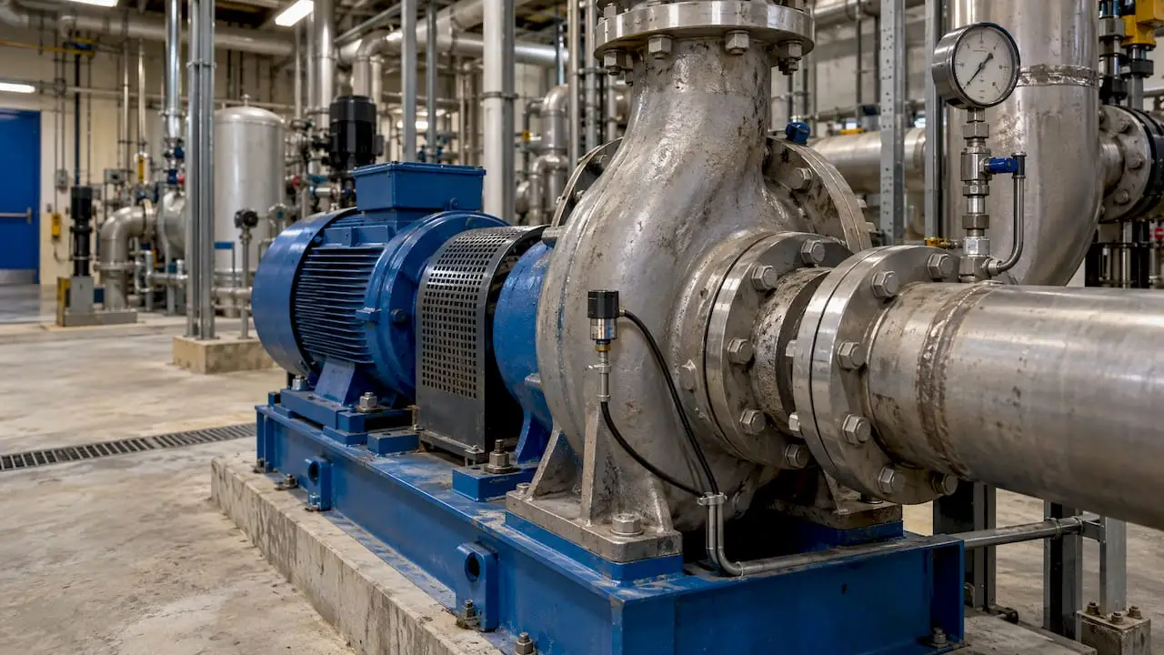
The unit is yours to choose. Lifetime can be counted in operating hours, cycles, distance or days. For a delivery fleet, kilometers or engine hours usually fit. For a pump, run hours. Pick the unit your maintenance schedule already uses.
RUL is an estimate, not a countdown. Prognostics literature treats it alongside time of failure and probability of failure as the core prognostic outputs. A statistical RUL is a distribution: “most likely 400 more hours, and a 10% chance of failing before 250” is a more honest and more usable statement than “400 hours.”
The statistical form is simple. A 2024 survey of deep-learning RUL methods writes it as RUL = T − t, where T is the failure time and t is how long the asset has survived so far. All the difficulty lies in estimating T for an asset that has not failed yet.
How RUL is calculated: the three main approaches
There is no single formula for the whole field. The right approach depends on what history you have. A widely used technical overview groups the methods into three families: survival, similarity and degradation models. The table below puts them side by side.
| Approach | What it needs | How it estimates RUL | Typical fit |
|---|---|---|---|
| Survival model | Historical lifetimes and failure or replacement records, plus covariates such as load or age | Fits a probability distribution or proportional-hazards model to lifetimes and updates it with current condition | Fleets of similar assets with a decent failure history |
| Similarity model | A library of run-to-failure degradation profiles | Matches the asset’s current sensor trajectory to the closest historical profiles and reads off their remaining life | Many assets that have been run to failure, with rich sensor logs |
| Degradation model | A condition indicator that trends over time and a defined failure threshold | Extrapolates the indicator until it crosses the threshold | Assets maintained conservatively, where run-to-failure data does not exist |
Survival models
Survival models use the lifetimes you have already recorded. They fit a distribution to how long similar assets lasted, and proportional-hazards versions let conditions such as vibration levels or oil chemistry raise or lower the risk. A Canadian case study on haul-truck wheel motors used this idea on nine years of oil-analysis data from 55 units. A proportional-hazards model identified which of 19 monitored elements, plus sediment and viscosity, mattered most, and fed a continue-or-overhaul decision with an RUL estimate per unit. The authors identified a potential 20 to 30% saving in overhaul costs against existing practice.
The lesson for a fleet: survival models reward the discipline of recording failures and replacements consistently. If your work-order history is patchy, fixing that is the first step.
Similarity models
Similarity models compare an asset’s current sensor data with profiles from assets that ran all the way to failure. They work well when you have many such profiles, which is common for components that are routinely run to failure, such as consumables, and rare for safety-critical equipment you replace early.
Degradation models
Degradation models are the natural choice when failure data is scarce, which is the usual case in well-maintained operations. You pick a condition indicator, such as bearing vibration or pump temperature, model how it trends, and project when it will cross a limit that defines failure. One published example sets limits on pump liquid temperature and pressure and forecasts when the indicator reaches them. Several sensors can be fused into one indicator with techniques such as principal component analysis, which is the idea behind our work on sensor data fusion.
Hybrid models
When neither physics nor data is enough alone, teams combine them. A 2022 study on turbomachine rotor blades paired a physics-based crack-growth model with Gaussian process regression and an unscented Kalman filter, and reported that the hybrid outperformed physics-only and data-only methods. A PHM Society paper on rubber-metal vibration isolators, used in railways, trucks and wind turbines, combines particle filtering with machine learning because little run-to-failure data exists for those parts. Hybrids cost more to build, so they pay off on expensive or critical assets.
The data an RUL model needs
Most RUL projects succeed or fail on data, not on the algorithm. Here is what to line up before anyone tunes a model.
- A clear failure definition. “Failure” might mean breakdown, a performance limit, or the point where you would replace the part. The Canadian National Research Council’s guide to condition-based maintenance stresses that a degradation measure must relate the asset’s state to remaining life and come with a defined failure threshold. Without that threshold, there is nothing to count down to.
- Condition data at a useful frequency. The same guide describes vibration monitoring as a common method for detecting wear, fatigue, misalignment and loose assemblies in bearings, gearboxes, pumps, motors and engines. Oil analysis, temperature, pressure, current draw and telematics fault codes are the other usual sources.
- Maintenance and failure records. Dates, hours, what was replaced and why. This is the raw material for survival models and for checking any model afterward.
- Operating context. Load, route, ambient temperature and duty cycle, because RUL depends on future use.
Health indicators
Most modern pipelines convert raw signals into a health indicator, a single number that tracks wear. The same 2024 survey describes a three-stage flow: preprocessing (filtering, normalization, splitting), health indicator generation, then RUL prediction. It lists three properties of a good indicator:
- Monotonicity: it does not recover on its own, since a worn part does not heal.
- Trendability: it follows the same general shape across assets.
- Prognosability: failures happen at a consistent indicator value.
An indicator that fails these tests will make any model look worse than it is. Checking them early saves weeks.
Judging whether an RUL model is any good
A model that fits history is not necessarily one you can schedule work around. Evaluate three things.
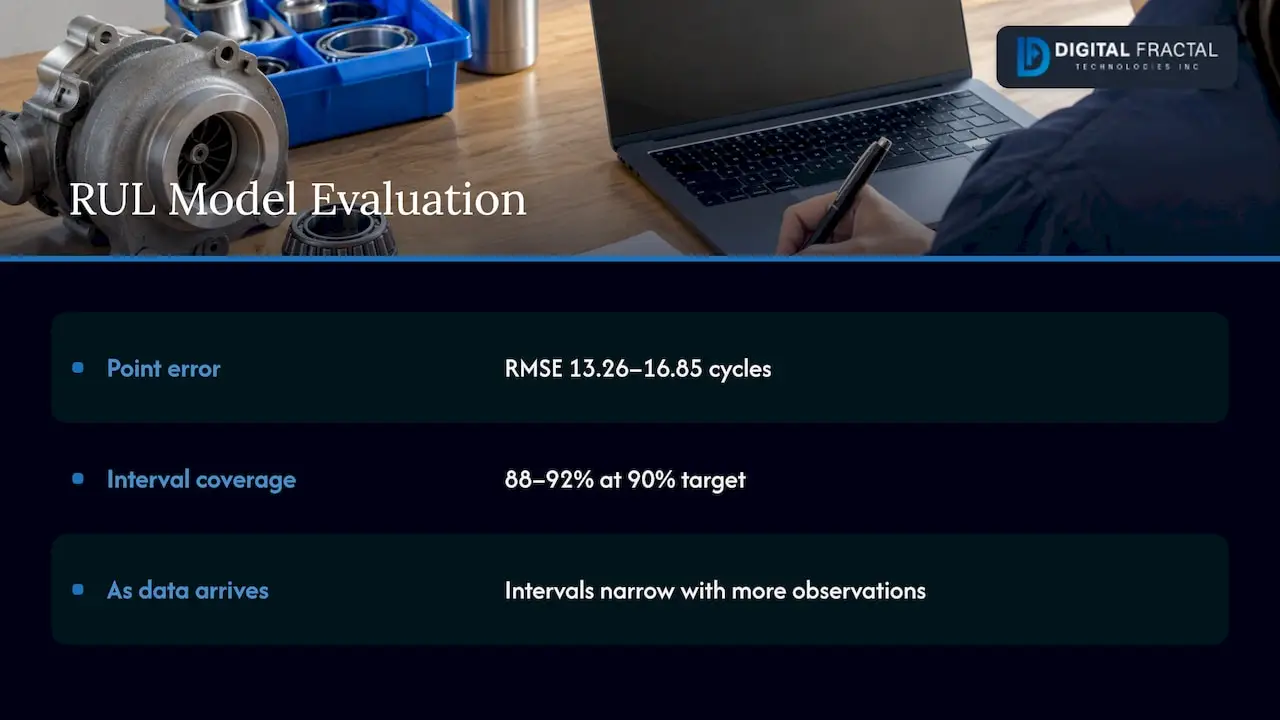
Point error. How far off is the estimate on average? On NASA’s C-MAPSS turbofan benchmark, a 2026 aircraft-engine study reported test RMSE (root mean square error, in cycles) between 13.26 and 16.85 across the four subsets. Benchmarks like this are useful for comparing methods, but your assets will behave differently, so your own error numbers matter more.
Interval coverage. If a model says it is 90% sure, it should be right about 90% of the time. The same study reported empirical coverage of 88 to 92% at a 90% target, and deliberately allocated its misses toward the safe side, avoiding overly optimistic predictions that would delay maintenance. That asymmetry is a good habit: late warnings usually cost more than early ones.
Behavior as data arrives. A Chapman University study on battery aging showed prediction intervals that were wider when only half the observations were available and narrowed as more data came in. That is the pattern you want: honest uncertainty that shrinks with evidence.
Evaluating when nothing has failed
Preventive maintenance is designed to stop failures, so you rarely see end of life. A 2026 PHM Society paper on evaluation addresses this directly: when ground truth is unavailable, predictions can be assessed retrospectively against the asset’s later sensor state, with results aggregated into a service-level indicator. In practice, that means you can keep scoring a live model even in a plant that seldom breaks down.
Ensembles and uncertainty
Combining several model families can reduce error. An EWSHM 2026 paper combined six model types across 100 hyperparameter configurations. Because the families make different kinds of mistakes, weighting them partly cancels errors, and disagreement between configurations serves as a measure of uncertainty. On a held-out C-MAPSS engine, the authors reported an RMSE of 3.73 cycles. Treat that as a single benchmark result rather than something to expect on your equipment.
From estimate to decision
An RUL number has no value on a dashboard nobody acts on. The aim is a rule such as: if the lower bound of RUL falls below the time to the next planned outage, schedule the work now.
The National Research Council describes condition-based maintenance as monitoring an asset’s condition continuously with installed sensors until evidence of deterioration appears, then maintaining it in time to prevent imminent failure. It notes this lowers overall maintenance cost and improves availability compared with fixed-interval preventive maintenance. It also separates this from predictive maintenance that relies on periodic, often manual, data collection.
A Canadian pulp mill pump study showed the decision logic. The expected remaining-life estimate and its confidence level helped managers choose between running a pump to the next scheduled outage or acting sooner, using green, caution and danger zones. Mapping RUL ranges to a few clear actions is what makes a model usable on a shop floor.
For a logistics operation, a working decision layer usually has three parts:
- Thresholds by consequence. A tractor unit on a long haul justifies a more conservative threshold than a yard truck.
- Links to scheduling. The estimate triggers a work order and a parts check. Our pieces on spare parts forecasting and AI-driven maintenance software cover that handoff.
- A feedback loop. Every completed repair becomes a labeled example that improves the next estimate.
If you need the business case first, see how to build a finance-ready ROI from a 90-day pilot, and for fleets in particular, our pilot-first approach to predictive maintenance in logistics.
Where RUL projects get stuck
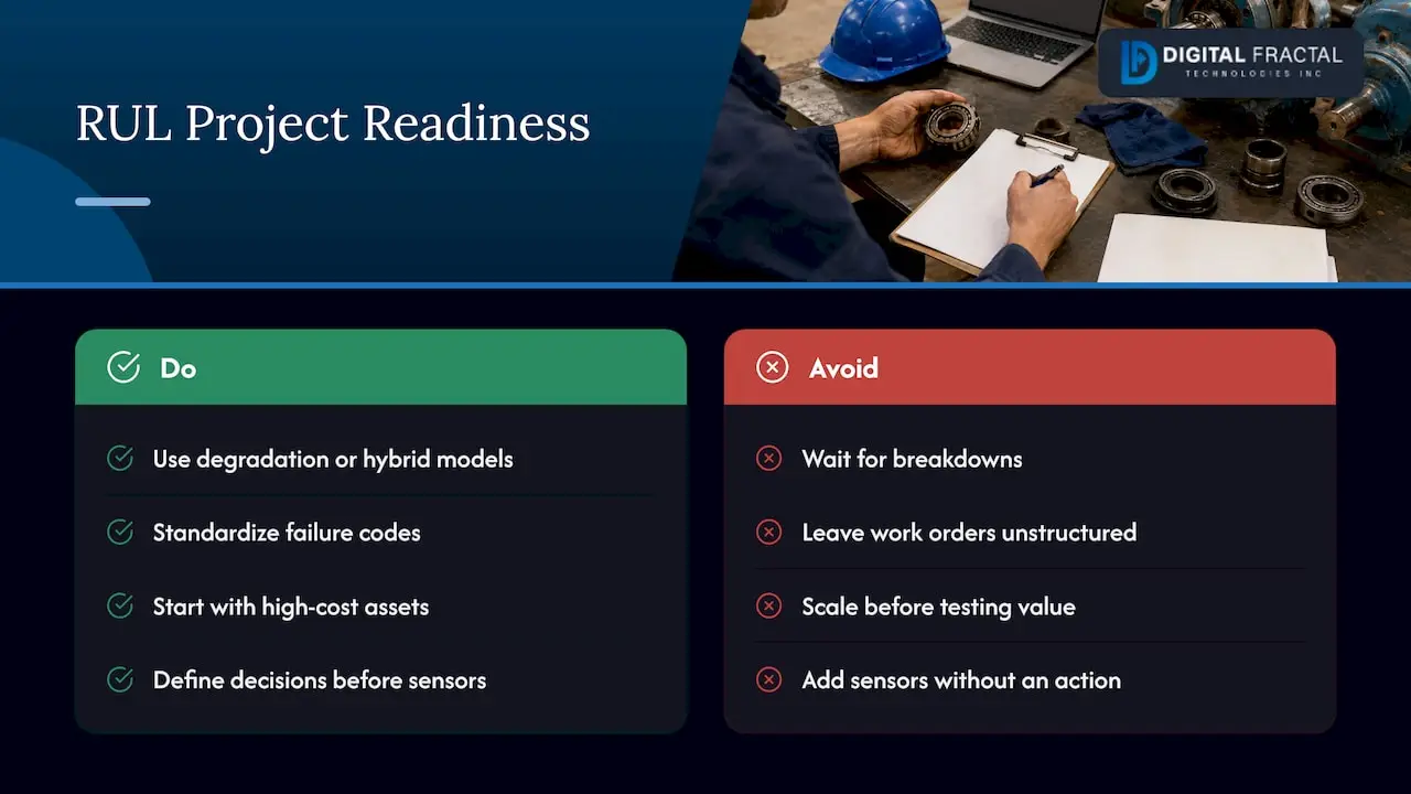
No failure labels. Well-run operations replace parts before they fail. Start with degradation or hybrid models, and use retrospective evaluation instead of waiting for breakdowns.
Inconsistent records. Free-text work orders and missing hours make survival models unreliable. Standardizing failure codes is cheap and pays off quickly. A structured look at this is in our guide to enterprise data readiness.
Too many assets at once. Models tuned on one asset class rarely transfer cleanly to another. Starting with a small, high-cost set of assets gives a clean test of value before scaling.
Sensors without a plan. Adding sensors before defining the failure threshold and the action produces data nobody uses. Decide the decision first, then the data.
Estimates nobody trusts. Operators accept a model faster when they can see why it flags an asset. Showing which indicators moved is more persuasive than a score.
How we help
We start with the AI Readiness Audit, a one-off engagement priced from $2,500 to $10,000. It identifies where automation and prediction will pay off in your operation, whether that is logistics, construction or oil and gas, so the first RUL model targets assets and decisions that matter. Our solutions are tailored to your workflows, systems and goals rather than off-the-shelf, and we aim to deliver tangible business transformation within 90 days. When you are ready to build, our AI consulting and machine learning solutions cover discovery, implementation and build out.
If your maintenance decisions currently rest on calendar intervals and experience alone, an audit is the quickest way to see which assets have the data to support RUL modeling now and which need groundwork first.
Our perspective
Most RUL projects we would want to take on begin with a decision, not a model. Ask what your planner would do differently on Monday if they knew an asset had 300 hours left instead of 600. If nothing changes, the model is a science project.
We favor starting small: a short list of costly assets, a clear failure definition, and a model simple enough that your technicians can see why it raised a flag. That is why we pair the AI Readiness Audit with a 90-day horizon. It forces the work toward something running in your operation, wired into your scheduling and your systems, rather than a report.
Generic tooling rarely survives contact with a real fleet or a real plant. Duty cycles, sensor quirks and maintenance habits differ, and the model has to be fitted to them. Our solutions are built around your workflows and goals for exactly this reason.
Souhail
FAQ
How is RUL calculated?
In statistical terms, RUL is the failure time minus the time the asset has already survived. Because the failure time is unknown, it is estimated by one of three routes: a survival model on lifetime history, a similarity match against run-to-failure profiles, or extrapolating a degradation indicator to a failure threshold. The result is best reported as a range with a probability.
What is the difference between RUL modeling and RUL estimation?
In practice the terms are used interchangeably. Modeling usually refers to building the mathematical or machine-learning model, and estimation to the number or range it produces for a specific asset at a specific time. Both depend on the same data, failure definition and evaluation.
How much data do I need?
It depends on the approach. Survival and similarity models need many lifetimes or run-to-failure profiles. Degradation models can work with a trending indicator and a defined threshold on far fewer assets, which suits operations that replace parts early. An audit of your records shows which route is realistic.
Can RUL modeling work for a mixed fleet?
Yes, but it is usually built asset class by asset class, because duty cycles and failure modes differ. Starting with the highest-cost class and expanding once the decision rules work is the lower-risk path.
Sources
- Introduction to Prognostics (PHM Society tutorial)
- An Introduction to Data-Driven Prognostics of Engineering Systems (PHM Society)
- Remaining Useful Life Prediction Based on Deep Learning: A Survey (PMC)
- Three Ways to Estimate Remaining Useful Life for Predictive Maintenance
- Optimizing a Mine Haul Truck Wheel Motors’ Condition Monitoring Program
- A hybrid framework for remaining useful life estimation of turbomachine rotor blades
- Hybrid Prognosis Method for Remaining Useful Lifetime (PHM Society)
- Condition-based Maintenance Management in Critical Facilities (National Research Council Canada)
- Remaining Useful Life Estimation for Aircraft Engines (IJPHM)
- Joint Modeling of Degradation Signals and Time-to-Event Data (Chapman University)
- Evaluation of Remaining Useful Life Prediction Algorithms (PHM Society)
- Robust Ensemble Framework for Extrapolation and Uncertainty (EWSHM 2026)